Our project presents physically accurate rendering and simulation of thin-film materials (specifically bubbles). In particular we produced realistic videos showcasing the varying iridescence and movement of bubble surfaces.
The project consists of four components
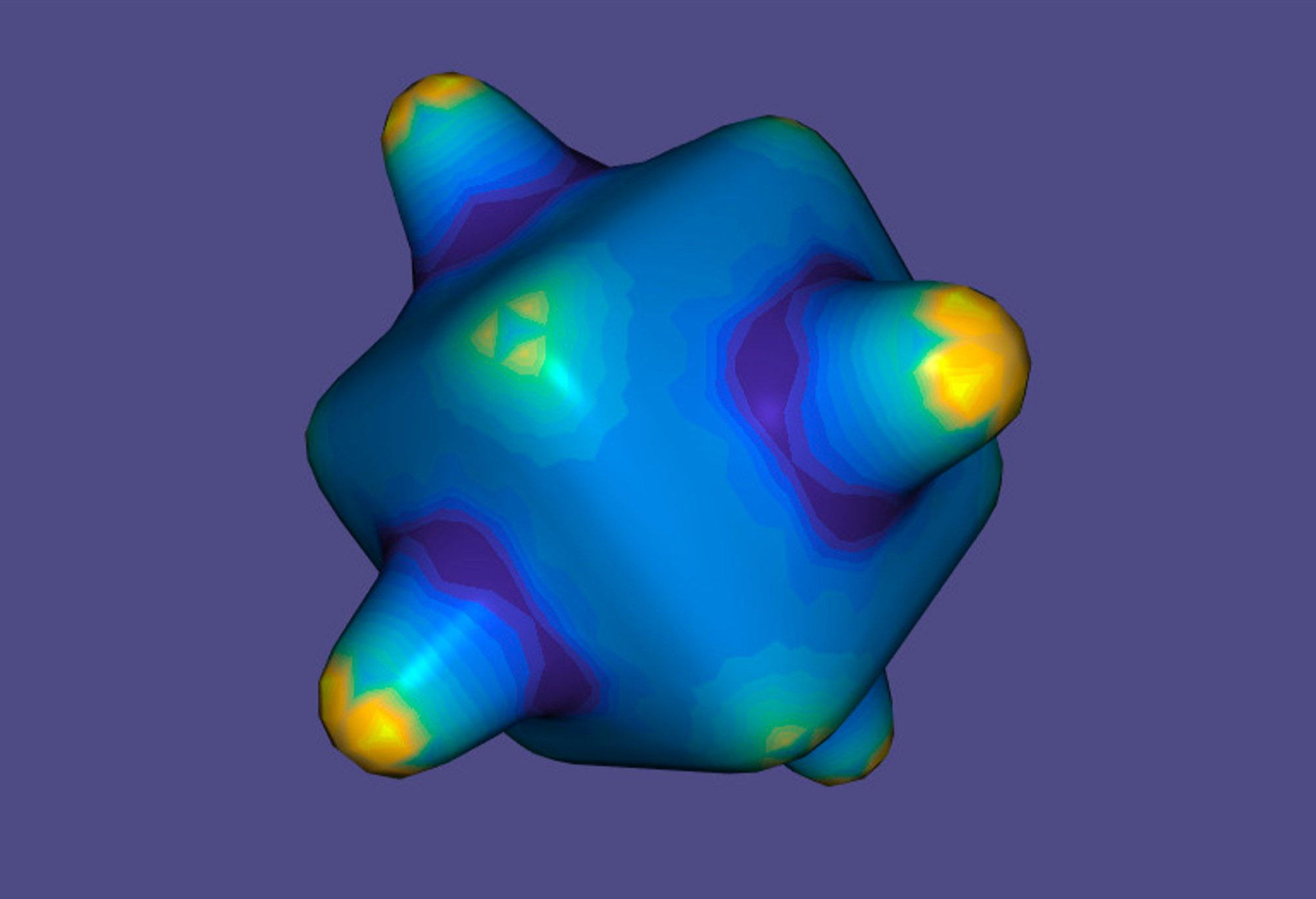
.obj file at a constant time interval so it could be ingested by the renderer and rendered in a scene.The first part of the project was bubble mesh generation and simulation. We borrowed the geometric approach from Ishida’s 2017 paper “A Hyperbolic Geometric Flow for Evolving Films and Foams”. The core idea behind it is a mean-curvature flow, where surface points are accelerated along their normal depending on the mean curvature at those points. This captures the idea that bubbles in the real world tend to minimize their surface area due to surface tension. Points where the bubble is bulging outward get pushed in, and points where the bubble is sunken in get pushed outwards.
Specifically, the equation of motion is given below, where $H$ denotes mean curvature, $\mathbf{n}$ denotes surface normal, $\Delta p$ is a term describing the internal pressure of the bubble, and $\beta$ is a constant relating to the bubble’s surface tension coefficient.
$$\frac{\mathrm{d}^2\mathbf{x}}{\mathrm{d}t^2} = -\beta H(\mathbf{x},t)\mathbf{n}(\mathbf{x},t) + \Delta p\mathbf{n}$$
Hyperbolic geometric flow on its own, corresponding to the left term of the equation, doesn’t preserve enclosed volume of the bubble, so the corrective term \$\Delta p\mathbf{n}\$ is added to remedy this. In practice, the simulator doesn’t calculate \$\Delta p\$ directly, and simply tries to ensure that the enclosed volume is constant by adjusting the mesh after each timestep.
To discretize the continuous hyperbolic geometric flow, we follow Ishida in using a triangle mesh and the well-studied discretization of mean-curvature for triangle meshes to implement the dynamics.
$$H_N = M^{-1}LX$$
Where $M$ denotes mass matrix, $L$ the cotangent matrix, and $X$ the vertex positions. This discretization upholds an important invariant studied in differential geometry (Gauss-Bonnet Theorem) and is widely used in computer graphics.
Ishida’s work goes much farther in extending this flow to non-manifold geometry, replacing mean-curvature normal with a variational surface area functional and a means of computing it on a triangle mesh.
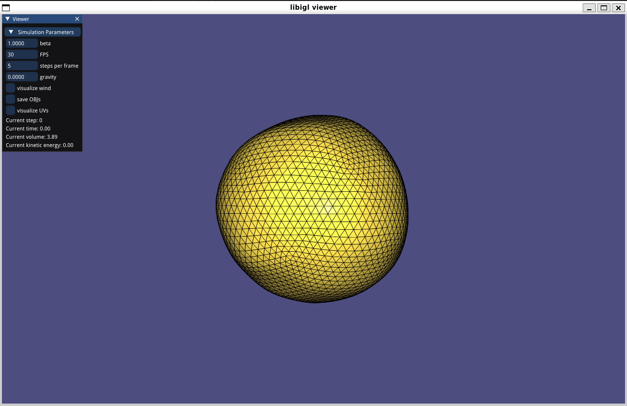
These dynamics were implemented using the libigl framework, which provides OpenGL skeleton rendering code and a variety of geometric / mesh processing operations to speed up prototyping. The C++ Eigen library was used to perform linear algebra operations.
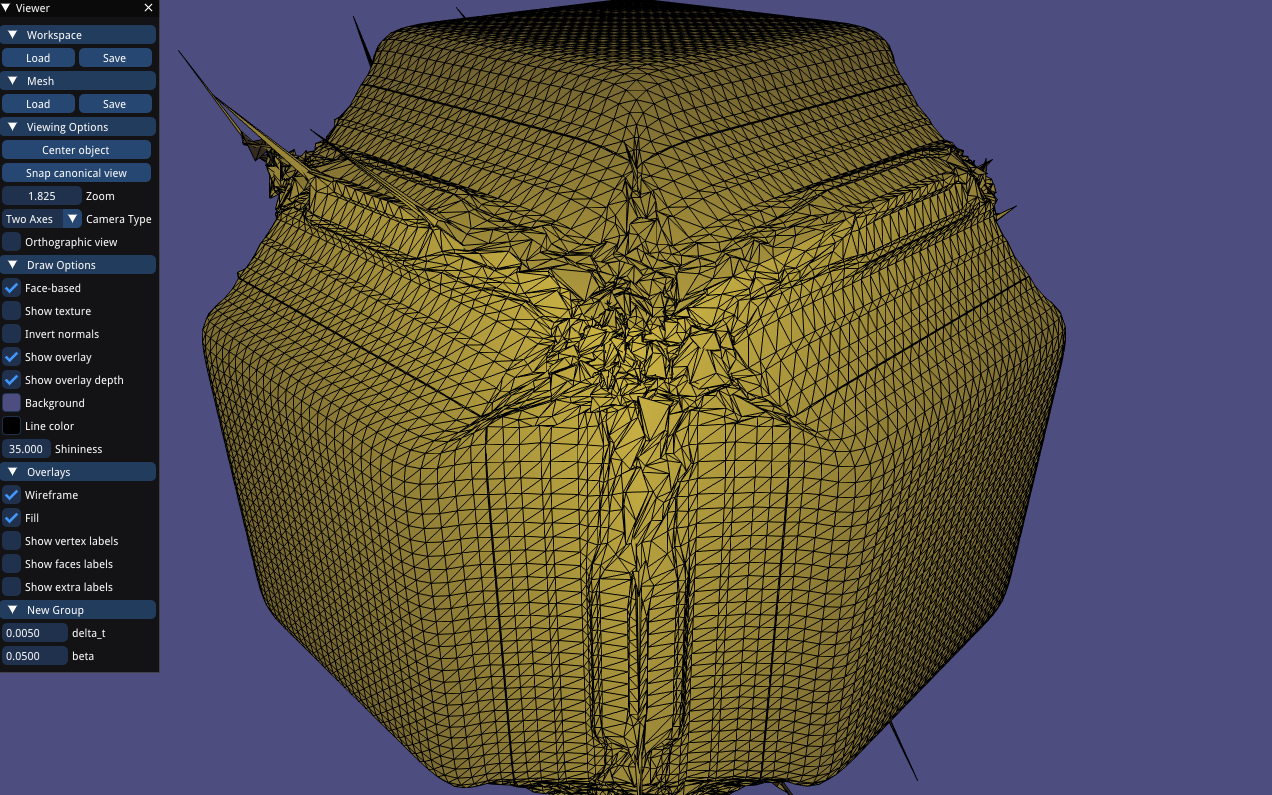
To preserve numerical stability while running the simulation, we have to periodically remesh and remove degenerate geometry. We used an external library which performs isotropic remeshing, modifying it to prevent volume loss during projection step after tangential Laplacian smoothing as well as hooking into its edge-split and edge-collapse routines to interpolate velocity of newly created geometry.
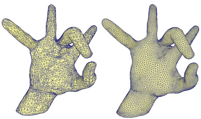
Ishida’s paper utilizes a software package known as LosTopos for this purpose, as it supports multimaterial, non-manifold surface tracking and remeshing. Unfortunately, lack of documentation and time meant we were unable to pursue this route.
We also included two external forces within the simulation: wind and gravity. A wind field was created by computing the curl of a vector potential using 3 components of 3D Perlin Noise
$$\Psi = (n_x, n_y, n_z)$$
$$\mathbf{F}_{wind} = \nabla \times \Psi$$
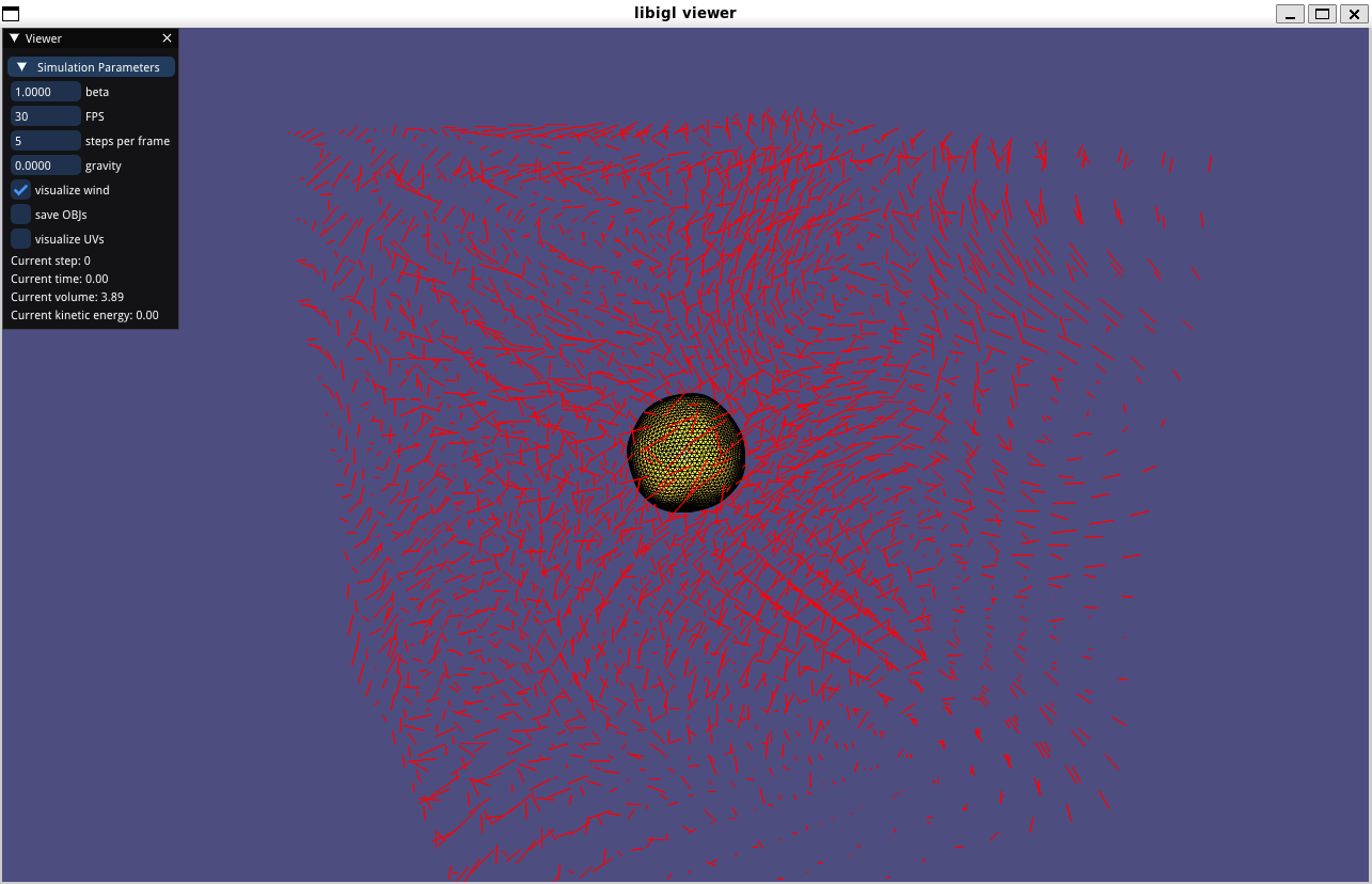
By the identity $\nabla \cdot (\nabla \times \mathbf{A}) = 0$, we know that $\mathbf{F}$ is divergence-free, which is expected due to incompressibility of air. Along with gravity, $\mathbf{F}_{wind}$ is coupled into bubble dynamics during sympletic Euler integration ($\vec{v}_{t+1} = \vec{v}_t + \vec{a}_t\Delta t$, $\vec{x}_{t+1}=\vec{x}_t+\vec{v}_{t+1}$) as part of $\vec{a}_t$.
Finally, we implemented a small .obj export module so the resulting meshes could be used within our pathtracer.
Future Extensions
A future extension would be implementing multi-bubble systems and interactions. Unfortunately, the nature of non-manifold meshes makes them hard to operate on, so it might be interesting to pursue a point-based method instead, where the mesh surface is instead discretized as a point cloud. This is the approach taken in many recent bubble simulation papers based on the SPH method of Computational Fluid Dynamics, but hasn’t been explored with the geometric-flow based bubble simulation approach described here. Methods for computing surface normals (using essentially PCA), mean curvature, and volume (”shrink-wrapping”) exist for point clouds, so in principle Hyperbolic Geometric Flow could be extended to that domain. Doing so avoids the need for costly remeshing operations and the general headache of working with non-manifold meshes. We were unable to explore this due to time constraints.
In order to accurately render the bubble we relied on ray tracing. We extended the Pathtracer code implemented in Homework 3. The main challenge in realistically rendering thin-film objects was in describing a BSDF class that can handle the reflectance and refracting dynamics of thin-film materials.
The underlying physics of thin-film interference is what gives them their vibrant colors. Specifically, the wave nature of light interacting with an optical medium leads to interference effects, as shown by this diagram
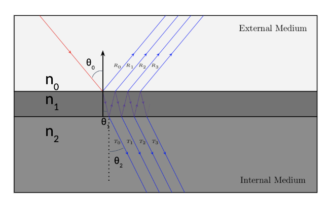
Each incoming ray of light can bounce and transmit multiple times. Since we assume $d$ (thickness of bubble) is on the order of nanometers, approximating this using a BSDF is still reasonable, but we need to include the contribution of $R_0$, $R_1$, $R_2$, etc. in the reflectance term and correspondingly $T_0$, $T_1$, etc. in the transmittance term.
The physically accurate way to compute the contribution of these bounces is using Fresnel Coefficients and Airy Summation. Fresnel coefficients describe the change in amplitude and phase of the electromagnetic waves at a boundary between two optically different mediums, and are derived from solving plane-wave solutions of Maxwell’s Equations.
$$\begin{align*}
r_s &= \frac{\eta_1\cos\theta_1 - \eta_2\cos\theta_2}{\eta_1\cos\theta_1 + \eta_2\cos\theta_2} \\
t_s &= \frac{2\eta_1\cos\theta_1}{\eta_1\cos\theta_1 + \eta_2\cos\theta_2} \\

r_p &= \frac{\eta_2\cos\theta_1 - \eta_1\cos\theta_2}{\eta_2\cos\theta_1 + \eta_1\cos\theta_2} \\
t_p &= \frac{2\eta_1\cos\theta_1}{\eta_2\cos\theta_1 + \eta_1\cos\theta_2} \\
\end{align*}$$
Where $\eta$’s are indices of refraction, $\theta_1$ and $\theta_2$ are incident and transmitted angles respectively (calculated using Snell’s Law). Note that these coefficients can be complex valued, and in the cases of total internal reflection or conductors, these equations are not fully accurate (but this is not a concern for our basic case of a dielectric between two layers of air), describing a phase shift.
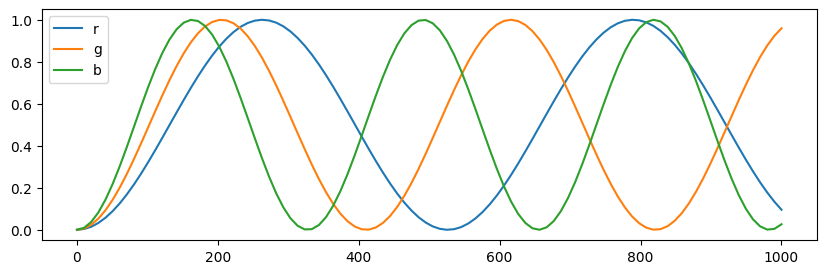
Refraction and distance traveled (the “optical path difference”) changes the phase of the light for each subsequent reflection and refraction. If two reflections are $180^\circ$ out of phase, then they will destructively interfere, so light of that wavelength have lower reflectance.
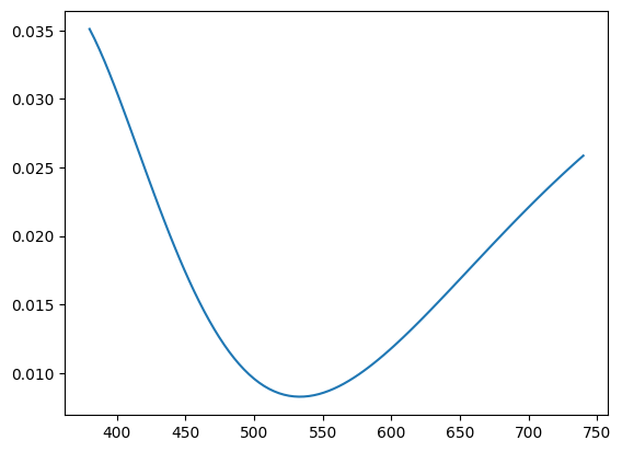
$\eta=1.33$. Incident medium has $\eta=1$, transmitting media has $\eta=1.2$, and incoming ray is at normal incidence and $S$-polarized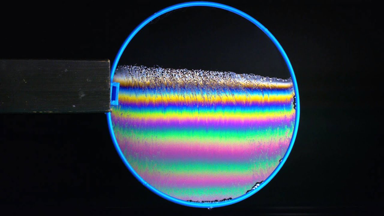
To capture contribution of all the number of bounces, we compute the Airy summation, which just adds up all of the difference bounces, adding a factor of $r_{12}r_{23}e^{-2i\phi}$ with each one. $r, t$ are the Fresnel coefficients from earlier and $e^{-2i\phi}$ is the phase shift due to optical path difference. Since one light wave travels different distance than the other, the two move out of phase proportional to distance traveled, which is both angle and wavelength dependent. Because of the representation as complex numbers, this simple expression captures destructive and constructive interference effects.
$$r = r_{12}+t_{12}r_{23}t_{21}e^{-2i\phi}+t_{12}r_{23}(r_{12}r_{23})t_{21}e^{-4i\phi}+\cdots$$
$$t = t_{12}t_{23}e^{-i\phi}(1+r_{23}r_{21}e^{-2i\phi}+(r_{23}r_{21}e^{-2i\phi})^2+\cdots)$$
$$\phi = \frac{2\pi}{\lambda}\eta_2d\cos\theta_2$$
We can rewrite these as geometric series
$$r = \frac{r_{12}+r_{23}e^{-2i\phi}}{1+r_{12}r_{23}e^{-2i\phi}}$$
$$t = \frac{t_{12}t_{23}e^{-i\phi}}{1+r_{12}r_{23}e^{-2i\phi}}$$
To convert this into reflectance and transmittance intensities, we just take their square magnitudes $\lvert r \rvert^2$ and $\lvert t\rvert^2$. We make a simplifying assumption (made by most raytracers, especially production ones) that light is unpolarized, so simply taking the average of reflectance / transmittance for $S$ and $P$ polarized light is sufficient.
Much of the implementation required carefully translating the physical equations that govern the intensity of reflection and refraction that happens in thin-film objects as described above into code for the newly created BubbleBSDF class. Since the direction of the transmitted ray and reflected ray are governed by the incident direction and the IOR values of the thin-film, this would be a delta BSDF.
At a high level, we implemented functions that would give the reflectance at a point given the wavelength of the ray, thickness of the film at the point, and the $\eta$ values of the film. We sample one wavelength per color channel (at 700nm, 546.1nm, and 435.8 nm, where the values of the RGB color matching functions achieve their maximum) Once we get these reflectance and transmittance values at our intersection point, the next issue is actually choosing whether to sample the transmitted ray or the reflected ray as the next bounce. This decision was made by simply probabilistically by choosing the ray proportional to the intensity (i.e. importance sampling based on reflectance / transmittance values).
$\eta$ parameters as earlier plotInterestingly, the current BSDF implementation is general enough to get transmittance and reflectance values at arbitrary $\lambda$, $d$, and $\eta$ values, leaving room for more complex rendering techniques, where the thickness of the surface is varying (possibly informed by underlying bubble simulation using Lagrangian advection of thickness like [Ishida 2020] or an SPH solver approach like MELP), or sampling a spectrum of wavelengths instead of just a constant wavelength for each color channel, and finally having different type of thin-film surfaces (by varying the $\eta$ value).
Future Extensions
Our current strategy of sampling just one wavelength to determine the reflectance / transmittance in RGB spectra is not very physically accurate, as demonstated by [Belcour and Parla 2017], often leading to out-of-gamut colors and clipping. Ideally, we would convert the class pathtracer to perform semi-spectral rendering like PBRT in order to maximize visual fidelity of thin-film material, but this was too out of scope / time-consuming.
Additionally, varying the thickness of the film is also another way to get a lot more realism: incorporating the effect of gravity onto film thickness and the turbulent flow that occurs on the surface of the bubble can add an extra layer of depth to the visual realism.
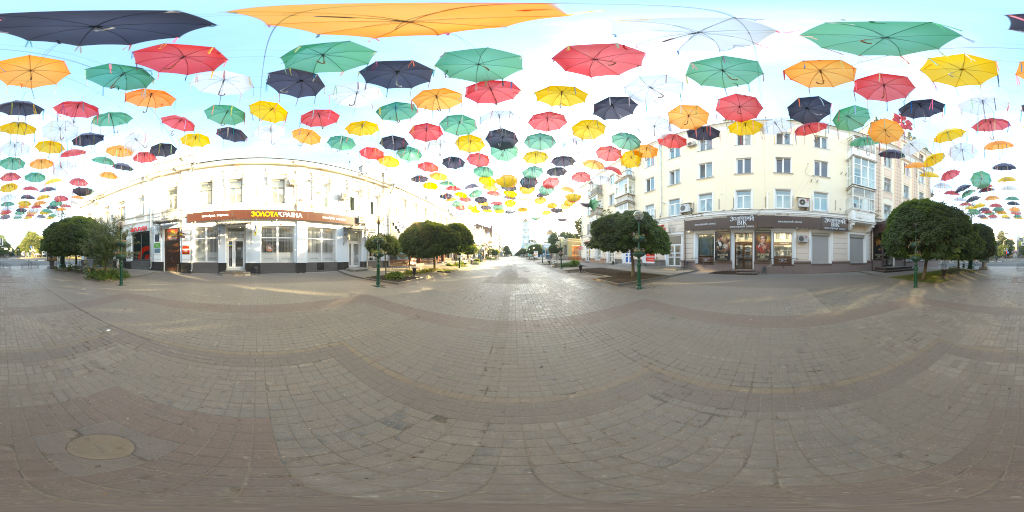
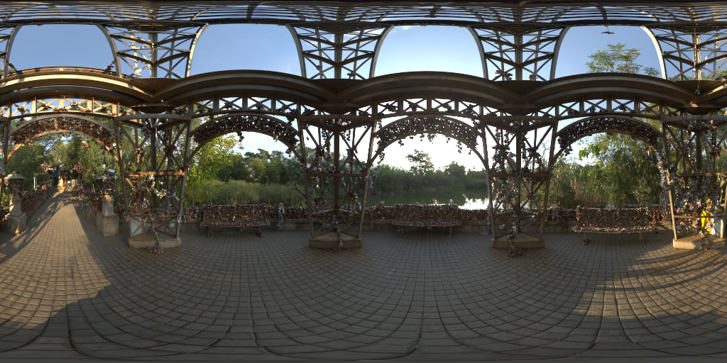
To create realistic and interesting lighting and reflections we opted for HDRi maps which hold real-world lighting data captured in high dynamic range in a spherically-projected 2D texture. Rather than being placed in a Cornell box, where the lighting effects are quite simple and thus lead to less interesting visual effects on the bubble, we thought it might prove more beneficial to use an environment map to create a more dynamic visual. This meant that we needed to also augment the Pathtracer to support environment lighting. Luckily the project 3-2 Pathtracer already had a lot of the skeleton to read in .exr files and apply the necessary setup required to map each point in the sampled environment space to a radiance value for the raytracer. All that needed to be implemented were a few functions that initialized the conditional and pdf probability valued data structures used in the sample_dir and sample_L functions when sampling out in a direction toward the environment map. It also turned out that the starter code did not have native support for environment map lighting sampling on delta BSDF functions so the main ray tracing method had to be augmented to provide the functionality, which finally gave a working environment map lighting feature to the Pathtracer.
In order to connect the mesh and the render portions of our code, we first use the mesh creation and re-meshing scripts to output object files. These object files do not hold transformation or camera rotation data, both important inputs into the renderer to get changing camera angle effects as well as the precise placement of the mesh in the rendering world space. As such we take those object files and put them through a custom written Python script that automates the entire pipeline, turning them into .scene files, which then attaches metadata, including transforms and camera positions, to the already existing object data. This script also changes the formatting of this information so that the pathtracer is able to use it. The pathtracer thus takes in this object data, transforms the given object, and then applies the render function to it. The python script, runner.py also takes care of running this rendering loop for every single object file that exists in the directory, automating the need to invoke the Pathtracer for every frame we need to render with the necessary arguments that include outputting to a specified filename. In this manner, we could just run the python program and then later as a postcondition expect the output directory to be populated with all the rendered scene images. Finally, to produce the nice looking videos, we took the rendered frames and then imputed them into the CLI tool ffmpeg to get the final output video, completing the entire pipeline.
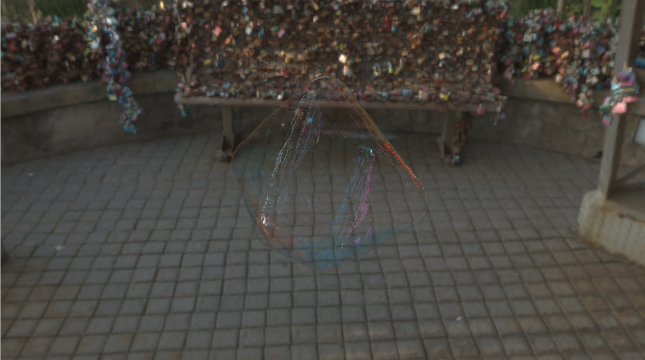
This was one of our rendered images of a bubble during a specific transformative time step, which uses a cube-shaped bubble as the initial starting point. The background uses the HDRi map mentioned earlier.
These are additional videos showcasing bubble with some denoising and camera spin
[1] Sadashige Ishida, Masafumi Yamamoto, Ryoichi Ando, and Toshiya Hachisuka. 2017. A Hyperbolic Geometric Flow for Evolving Films and Foams. ACM Trans. Graph. 36, 6, Article 199 (November 2017), 11 pages. https://doi.org/10.1145/3130800.3130835
[2] Laurent Belcour and Pascal Barla. 2017. A Practical Extension to Microfacet Theory for the Modeling of Varying Iridescence. ACM Trans. Graph. 36, 4, Article 65 (July 2017), 14 pages. http://dx.doi.org/10.1145/3072959.3073620
[3] Sadashige Ishida, Peter Synak, Fumiya Narita, Toshiya Hachisuka, and Chris Wojtan. 2020. A Model for Soap Film Dynamics with Evolving Thickness. ACM Trans. Graph. 39, 4, Article 31 (July 2020), 11 pages. https://doi.org/10.1145/3386569.3392405